
Every antenna engineer knows the moment. The simulation looks clean. The prototype comes back from the workshop. The measured result does not match. Is the model wrong, the prototype faulty, or the measurement setup off? The IEEE recommended practice for antenna measurements (IEEE Std 149-2021) addresses measurement uncertainty for a reason: a measurement only means something once you know what can distort it. The same is true of a simulation.
This article explains where simulation-to-measurement discrepancies come from, what you should actually compare, and how to build a correlation workflow. It draws on how Anyfields engineers designed and validated the antennas of the EMBox Lab starter pack.
In brief
- Simulation and measurement are two independent views of the same antenna. Agreement between them builds confidence; disagreement is information, not failure.
- Most discrepancies come from a short list of causes: material and geometry assumptions, feed modeling, fixtures and environment, measurement setup, and comparing quantities that are not truly equivalent.
- Comparing like with like matters most. The simulated output must match the measured quantity, plane, distance and normalization.
- Near-field maps reveal where a discrepancy originates. A single gain figure only tells you that one exists.
- In a documented case, a 2.45 GHz rectangular patch showed 5.85 dBi simulated gain versus 5.8 dBi measured.
Why compare antenna simulation with measurement at all?
Electromagnetic simulation predicts how an antenna should behave. Measurement shows how a real, manufactured antenna actually behaves. Neither is the full truth on its own.
A simulation is only as good as its inputs. Material properties, geometry, mesh and boundary conditions are all modeling choices. A measurement is only as good as its setup. Alignment, distance, cables and environment all leave a mark on the result.
Comparing the two gives you a cross-check. When an independent prediction and an independent observation agree, confidence in both increases. When they disagree, the gap points you toward something worth investigating: a modeling assumption, a manufacturing defect, or a measurement artifact.
This is why correlation is a standard step in antenna development, from early prototyping to integration on a platform. It is also why it is worth teaching: students who learn to read a discrepancy learn how engineering validation really works.
What exactly should you compare between simulation and measurement?
The most common correlation mistake is comparing two quantities that look alike but are not the same. Before reading any gap as a real discrepancy, check that both sides describe the same physical quantity, in the same place, in the same way.
Are you comparing far-field figures or near-field maps?
Far-field metrics are compact and familiar: gain, half-power beamwidth (HPBW), radiation pattern cuts. They are ideal for checking whether an antenna meets its specification.
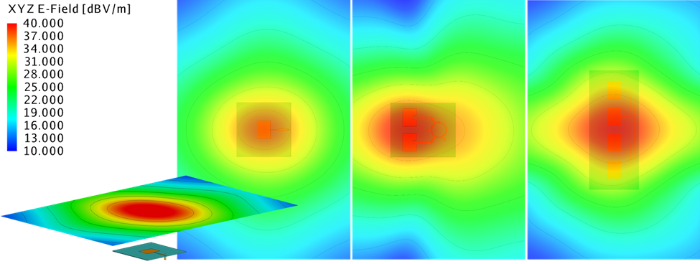
Near-field maps show the field distribution close to the antenna. They are richer. On an array, for example, a near-field map shows the contribution of each radiating element. A missing or weak element appears directly on the map, while it may only show up as a small change in a far-field figure.
The two levels are complementary. A far-field comparison tells you whether the antenna performs as expected. A near-field comparison helps you understand why it does or does not.
Is the simulated output the same quantity as the measured one?
Each measurement method observes a specific quantity. The simulation must export exactly that quantity. For example, the Anyfields infrared thermography method produces an E-field map: the amplitude of the total tangential electric field, in V/m, at the surface of a sensing film. A meaningful comparison therefore requires the simulated amplitude of the total tangential E-field, on a plane at the same position and distance from the antenna.
Comparing that map with a single field component, or with a field computed at another distance, produces a gap that has nothing to do with the antenna.
Are both results normalized and scaled the same way?
Patterns are often normalized to their maximum and displayed in dB. Check that both results use the same reference, the same scale (linear or dB), and the same input power assumption. Check the coordinate system and orientation too. A pattern rotated by 90° can look like a severe mismatch.
Where do simulation-to-measurement discrepancies come from?
Most discrepancies fall into five families. Some sit on the simulation side, some on the measurement side, and some come from the comparison itself. The table below is a practical starting point for diagnosis.
| Source | Typical symptom | What to check first |
|---|---|---|
| Material and geometry assumptions | Frequency shift, gain offset | Substrate permittivity and loss tangent at the working frequency, as-built dimensions, copper thickness |
| Feed and connector modeling | Mismatch, asymmetric pattern, unexpected sidelobes | How the port, connector and feed line are modeled; solder joints; cable routing |
| Fixtures and environment | Distorted pattern, ripples | Mounts, nearby metal parts, finite ground plane, reflections not present in the model |
| Measurement setup | Global offset, shifted or rotated map | Distance to antenna, alignment, orientation, input power, sensitivity limits of the system |
| Non-equivalent comparison | Mismatch that does not respond to any physical fix | Quantity, plane, normalization, scale and coordinate system (see previous section) |
Why do material properties cause so many gaps?
Substrate datasheets often give permittivity at a single frequency, with a tolerance. A small difference between the modeled and the real value shifts the resonance. On a narrowband antenna such as a patch, this alone can explain a visible gap in gain at a fixed frequency.
Why does the feed matter so much?
The feed is where the model and the real object diverge most easily. A simulation port is an idealization. The real antenna has a connector, a solder joint and a cable. On a multi-port antenna or an array with a feed network, small differences in amplitude or phase between paths change the radiated pattern.
How do you rule out the measurement setup?
Repeat the measurement. Move the antenna slightly and measure again. A discrepancy that changes with each setup points to the setup. A discrepancy that stays stable points to the antenna or the model. Every measurement system also has a sensitivity limit: with the Anyfields method, fields below about 200 V/m at the film surface cannot be distinguished from noise. Low-field regions must be read with that limit in mind.
How did Anyfields correlate simulation and measurement on the EMBox Lab antennas?
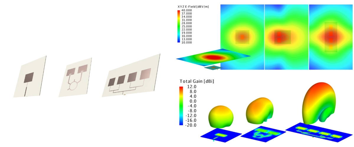
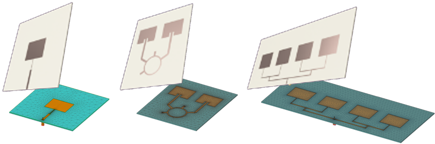
The EMBox Lab starter pack includes three antennas designed by Anyfields engineers for antenna teaching. Because they are used to demonstrate electromagnetic concepts in class, their measured behavior had to match their predicted behavior. They were therefore designed and validated through a full simulation-to-measurement loop.
| Antenna | Dimensions | Frequency | Concept illustrated |
|---|---|---|---|
| Rectangular patch | 12.5 × 12.5 cm² | 2.4 GHz | Basic radiation, gain, radiation pattern |
| Rat race 2-patch array | 15 × 12.5 cm² | 2.4 GHz (2 SMA ports) | Feed network, phase between elements |
| 4-element rectangular patch array | 27.5 × 11 cm² | 2.4 GHz | Array behavior, beam formation, phase and feed-network concepts |
What did the workflow look like?
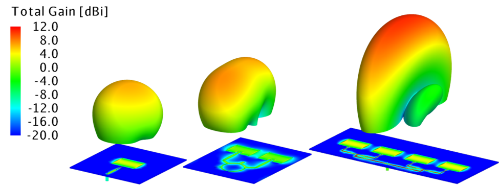
The antennas were modeled in Simcenter Feko, the electromagnetic solver used by the Anyfields team for this project. Before manufacturing, engineers predicted far-field radiation patterns, gain and surface current distributions, then refined the designs.
The team also computed the near-field electric field distribution around each antenna. This step is what makes the later comparison meaningful: it gives a simulated reference for the same kind of field map that EMBox Lab measures.
Once manufactured, each antenna was measured with EMBox Lab. The Compare function of the EMSoft software placed the measured near-field maps side by side with the simulated ones. EMSoft accepts imported results from several solvers, including HFSS, FEKO and CST, so the same workflow applies whatever simulation tool a team uses.
What results did the patch antenna give?
The rectangular patch, characterized at 2.45 GHz, is a documented reference case.
| Metric | Simulated | Measured |
|---|---|---|
| Gain | 5.85 dBi | 5.8 dBi |
| Half-power beamwidth (−3 dB) | ≈80° | 79.1° |
The measured far-field values were obtained with the EMSoft Far-Field function, which computes gain and HPBW from the near-field measurement. The agreement is close on both metrics.
What happens when the results do not match?
During development, some measured results did not match the initial predictions. Investigating these differences helped the team refine the antennas and improve the correlation.
On an array, this is where the near-field map is most useful. Each patch appears as a distinct region on the map. If one element radiates less than expected, the map shows which one, before you even look at the far-field pattern.
How do you set up a simulation-to-measurement correlation workflow?
A reliable correlation workflow is planned before the first measurement, not after the first mismatch. The steps below apply whatever solver and measurement method you use.
- Define the comparison upfront. Decide which quantities you will compare (gain, HPBW, pattern cuts, near-field map) and at which frequencies.
- Model what you will build. Use measured or supplier-verified material properties when you have them. Include the connector and the feed as realistically as possible.
- Export the matching quantity. Configure the simulation to output exactly what the measurement observes: same field quantity, same plane, same distance, same orientation.
- Document the measurement setup. Record distance, alignment, input power, frequency and fixtures. A setup you cannot reproduce cannot be debugged.
- Normalize consistently. Use the same reference, scale and coordinate system for both results before comparing.
- Compare at two levels. Start with far-field metrics to check performance. Use near-field maps to locate the origin of any gap.
- Investigate one hypothesis at a time. Change one parameter in the model, or one element of the setup, and check whether the gap moves.
- Record the outcome. Keep the final model, the measurement data and the explanation of each discrepancy. This becomes your reference for the next design.
Does a close match prove that both simulation and measurement are right?
Not on its own. A close match is strong evidence, but it is not proof. Two results can agree because both are right. They can also agree because they share the same wrong assumption, for example the same incorrect material value used to design the antenna and to interpret its measurement.
The value of correlation comes from independence. The simulation and the measurement should rely on different principles and different inputs. The more independent they are, the more their agreement means.
This is also why one good match is not enough to validate a method. Confidence grows with repeated agreement across several antennas, frequencies and configurations. It grows further when results can be cross-checked against another measurement method, such as a far-field range or a classic anechoic chamber. Each method brings its own strengths, and they reinforce each other.
A discrepancy, in contrast, is always informative. It tells you that at least one assumption needs a second look.
FAQ - Simulation versus measurement
How close is close enough between simulation and measurement?
It depends on the application, the antenna type and the uncertainty of both the model and the measurement. A tolerance should be defined before measuring, based on your specification and the known uncertainty of your setup. Defining it afterward makes almost any result look acceptable.
Can I skip measurement if my simulation is detailed enough?
A detailed simulation reduces risk, but it still describes an idealized antenna. Manufacturing tolerances, assembly, connectors and the integration environment only appear on a real object. Measurement remains the step that confirms the antenna you built behaves like the antenna you designed.
Can I trust the antenna datasheet instead of measuring?
A datasheet describes the antenna in the manufacturer’s test conditions. Once the antenna is mounted on your platform, nearby structures and materials can change its behavior. Measuring in your own configuration tells you how it performs in your system.
Does near-field measurement replace far-field measurement?
No. They answer different questions and complement each other. Near-field maps are well suited to diagnosis and fast iteration. Far-field ranges and classic anechoic chambers remain references for full characterization. Many teams use both at different stages of development.
Does the correlation workflow depend on a specific simulation software?
No. The principles apply to any full-wave solver. What matters is that the solver can export the quantity your measurement observes. The EMSoft Compare function, for example, imports results from HFSS, FEKO and CST.
Conclusion: what should you take away?
Simulation and measurement are not competing answers. They are two independent views of the same antenna. Correlating them is how you turn a design into a validated design.
The method matters more than the tools. Compare equivalent quantities. Document your setup. Use near-field maps to locate problems and far-field metrics to confirm performance. Treat every discrepancy as a lead.
Simulation tells you what should happen. Measurement tells you what did. Engineering happens in the gap.
RF engineer, antenna designer or R&D lead? Contact us to compare your own simulation results with a near-field measurement of your antenna, or explore EMBox XL for R&D and production testing.